
Scalable & Sustainable Computational Biology: Vectorization, Indexing Tricks, and Numba/Cython
![]()
Speeding up code is sometimes an overlooked aspect in the field of computational biology. Numerous constraints (multiple projects, thesis writing, pressure to publish, etc.) often lead many to write simple implementations of a given function, at the expense of efficiency. This is problematic as such code is not scalable, which can limit further discoveries done by other researchers. In this article, I will look at all tasks performed by a specific Python function I have designed, showing first an example of slow code, and then a suggestion of a faster implementation. I hope this will provide some tips to you to perform a scalable, more efficient, and environmentally friendly science!
The Task
During my research, I was assigned to implement a relatively simple function. We work with single-cell data that includes clonal barcodes. These barcodes allow us to group and identify cells that belong to the same lineage, as a barcode would be passed from the mother cell to all subsequent daughter cells. Clonal barcoding is a potent tool for studying early fate biasing and can be used as input for some tools to infer the fate of non-barcoded neighboring cells.
The most basic fate bias estimation between two fates in barcoded cells consists of counting the occurrences of the fates in each clone. We then compare these occurrences to the ones of other fates to statistically assign a fate bias.
More precisely, we will calculate the fate bias $f$ as follows:
$$ f = \frac{c_A}{c_A+{c_B}\times{\alpha}^{-1}} $$with $c_A$ and $c_B$ being the number of occurrences of our fates A and B in each clone, and $\alpha= \frac{\sum c_A}{\sum c_B}$ is the ratio of the sum of all observed clones for each fate.
To test of significance of fate bias, we will perform a Fisher exact test, with a 2x2 contingency table:
$$ \begin{align*} \begin{array}{|c|c|} \hline c_A & c_B \\ \hline \sum c_A & \sum c_B \\ \hline \end{array} \end{align*} $$While this task should not be compute-intensive, there are several good examples of slow and inefficient code that can be fixed. You will see that slowness is not only caused by slow calculation but also by data access!
The system used for benchmark
The numbers showed here come from tests with my MacBook Pro M2P 32GB.
I used python 3.10.13 and installed the following packages:
pip install cospar fast_fisher
Loading libraries and the data
import cospar as cs
import warnings
import scanpy as sc
import numpy as np
import pandas as pd
import time
sc.set_figure_params()
warnings.filterwarnings('ignore')
Quick overview of the data
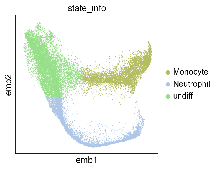
The data we will use here is a 30k+ cells dataset of mouse hematopoiesis. The cells were clonally barcoded once and then were subsequently sampled at multiple time points.
adata_orig = cs.datasets.hematopoiesis()
We will focus on the bifurcation between Monocytes and Neutrophils:
mask = adata_orig.obs.state_info.isin(["Monocyte","Neutrophil"]) | adata_orig.obs.NeuMon_mask
adata = adata_orig[mask].copy()
sc.pl.embedding(adata,color="state_info",basis="emb")
Some parameters needed
clone = 'X_clone' # key to access the clonal matrix
fA = 'Neutrophil' # fate A
fB = 'Monocyte'   # fate B
state_key = 'state_info' # key for fate assignments
cutoff = 0.01 # cutoff for Fisher test corrected p-values
Getting cell indices for each clone
We use a clone matrix saved in anndata under obsm as a sparse matrix, where the rows are cells and columns are clones. We need to extract which cell belongs to which clone. In other words, the task is to retrieve the row indices of each column.
def get_cellid_per_clone(adata,clone):
    X_clone = adata.obsm[clone]
    return [np.argwhere(X_clone[:,i])[:,0] for i in range(X_clone.shape[1])]
start = time.time()
cid = get_cellid_per_clone(adata,clone)
end = time.time()
print(f'{(end-start):.3}s')
0.756s
Why is this method slow? Though this approach is straightforward (practically one line), a for loop that calls np.argwhere for each of the columns implies that we are not leveraging NumPy’s ability to perform operations on entire arrays at once.
Let’s have a look at a faster implementation:
def get_cellid_per_clone_f(adata,clone):
    X_clone = adata.obsm[clone]
    # Extract and sort row and columns
    rows, cols = np.nonzero(X_clone)
    sort_idx = np.argsort(cols)
    rows_sorted = rows[sort_idx]
    cols_sorted = cols[sort_idx]
    # Get the count of unique columns
    _, counts = np.unique(cols_sorted, return_counts=True)
    # Split rows_sorted based on counts
    return np.split(rows_sorted, np.cumsum(counts[:-1]))
start = time.time()
cid = get_cellid_per_clone_f(adata,clone)
end = time.time()
print(f'{(end-start):.3}s')
0.00539s
Why is this fast? Because we use NumPy’s vectorized function np.nonzero to find the indices of non-zero elements in the entire array at once. Then, we sort these indices based on the column indices and split them into separate arrays for each column. By sorting the indices based on the column indices (np.argsort is also vectorized), the function avoids having to access the columns individually.
Getting the occurrence of our two fate labels in each clone
We want to count the occurrence of our two fate labels in each clone and the total of each fate. This involves retrieving the cluster assignment for each cell within each clone.
def get_counts_per_clone(adata,cid,state_key):
    # Convert cell id to assigned cell state for each clone
    cl = [adata[c].obs[state_key] for c in cid]
    # Count occurences of states per clone
    clA = np.array([(c==fA).sum() for c in cl])
    clB = np.array([(c==fB).sum() for c in cl])
    clAsum, clBsum = np.sum(clA) , np.sum(clB)
    return clA, clB, clAsum, clBsum
start = time.time()
clA, clB, clAsum, clBsum = get_counts_per_clone(adata,cid,state_key)
end = time.time()
print(f'{(end-start):.3}s')
1.71s
Why is this slow? Here the issue lies in the repeated access of the anndata object in a for loop, which is quite inefficient. Also, although this does not have that much of an impact, the function calculates the sum of clA and clB separately.
Here is a faster implementation:
def get_counts_per_clone_f(adata,cid,state_key):
    # Get cell id and clone id array
    i = np.repeat(np.arange(len(cid)), [len(c) for c in cid])
    c = np.concatenate(cid)
    cid_cl = np.column_stack((c, i))
    # apply cell/clone id array to states array
    df = adata.obs[[state_key]]
    df["clone"]=np.nan
    df.iloc[cid_cl[:,0],1]=cid_cl[:,1]
    # Count occurences of states per clone
    cnts = df.groupby(state_key).value_counts(["clone"])
    clAB = pd.concat([cnts[fA].sort_index(),cnts[fB].sort_index()],axis=1).values
    clA, clB = clAB[:,0], clAB[:,1]
    clAsum, clBsum = clAB.sum(axis=0)
    return clA, clB, clAsum, clBsum
start = time.time()
clA, clB, clAsum, clBsum = get_counts_per_clone_f(adata,cid,state_key)
end = time.time()
print(f'{(end-start):.3}s')
0.0103s
Why is this fast? First, we used vectorized functions np.column_stack and np.repeat to create a NumPy array assigning each cell index to a clone id. Then, we use the groupby method from pandas, which is optimized for grouping and aggregating data. Finally, the anndata is read and written only once, avoiding the usage of any for loop.
Calculating fate bias and its significance per cell
We will use the equation mentioned in the introduction, as well as the Fisher exact test. More precisely, we will perform the test on each clone using extracted counts of our two fates and their total sum.
def get_fate_bias(clA,clB,clAsum, clBsum):
    # Perform Fisher extact test on clone counts
    from scipy.stats import fisher_exact
    pvals = [fisher_exact(np.array([[cla,clb], [clAsum, clBsum]]))[1]
             for cla,clb in zip(clA,clB)]
    # Get fate biasing using clone counts
    slope = clAsum/clBsum
    fate_bias = clA/ (clA + clB/slope)
    return pvals, slope, fate_bias
start = time.time()
pvals, slope, fate_bias = get_fate_bias(clA,clB,clAsum, clBsum)
end = time.time()
print(f'{(end-start):.3}s')
1.17s
Why is this slow? Because scipy implementation of fisher_exact is written in plain Python. As this is the actual calculation part of our code, there should be room for improvement by using a faster implementation:
def get_fate_bias_f(clA,clB,clAsum, clBsum):
    # Perform Fisher extact test on clone counts
    from fast_fisher import fast_fisher_exact
    pvals = [fast_fisher_exact(cla,clb, clAsum, clBsum)
             for cla,clb in zip(clA,clB)]
    # Get fate biasing using clone counts
    slope = clAsum/clBsum
    fate_bias = clA/ (clA + clB/slope)
    return pvals, slope, fate_bias
start = time.time()
pvals, slope, fate_bias = get_fate_bias_f(clA,clB,clAsum, clBsum)
end = time.time()
print(f'{(end-start):.3}s')
0.0154s
Why is this fast? With a simple Google search, I found the Python package fast_fisher, which provides Numba and Python implementations of the Fisher exact test. Numba compiles a function using the LLVM compiler library, while Cython converts Python functions to compiled C code, both lead to great speedups.
Saving the data
One might think that saving data is a trivial task. Here is how to avoid inefficiencies!
def assign_results(adata,cid,pvals,fate_bias,cutoff):
    adata.obs["fisher_pval"] = np.nan
    adata.obs["fate_bias"] = 0.5
    for ci,p,f in zip(cid,pvals,fate_bias):
        adata.obs.loc[adata.obs_names[ci],'fisher_pval']=p
        if p < cutoff:
            adata.obs.loc[adata.obs_names[ci],'fate_bias']=f
start = time.time()
assign_results(adata,cid,pvals,fate_bias,cutoff)
end = time.time()
print(f'{(end-start):.3}s')
0.38s
Why is this slow? The function locates the index of the dataframe using adata.obs_names[ci] and assigns the values. This operation is not very efficient as it involves looking up the index for each element. In addition, loc is slow as the cell id needs to be converted into integer indexes.
def assign_results_f(adata,cid,pvals,fate_bias,cutoff):
    adata.obs["fisher_pval"] = np.nan
    adata.obs["fate_bias"] = 0.5
    c = np.concatenate(cid)
    # prepare assignment array
    cid_len = np.array([len(c) for c in cid])
    cid_pval_f = np.column_stack((
        c, np.repeat(pvals, cid_len),
        np.repeat(fate_bias, cid_len)
    ))

    # assign values to anndata
    col = adata.obs.columns
    adata.obs.iloc[cid_pval_f[:,0],col=="fisher_pval"] = cid_pval_f[:,1]
    cid_pval_f = cid_pval_f[cid_pval_f[:,1]<cutoff,:]
    adata.obs.iloc[cid_pval_f[:,0].astype(int),col=="fate_bias"] = cid_pval_f[:,2]
start = time.time()
assign_results_f(adata,cid,pvals,fate_bias,cutoff)
end = time.time()
print(f'{(end-start):.3}s')
0.00429s
Why is this fast? We prepare the assignment array outside the loop, which reduces the computational overhead. This assignment array is created by vectorized functions np.repeat and np.column_stack. To perform the actual assignment, we use iloc for indexing, which is faster than loc because it accesses the data directly by integer index. Lastly, we use boolean indexing (cid_pval_f[:,1]<cutoff) to filter the data, which is more efficient than using a loop.
Overall speed comparison
def slow_implementation(
    adata,
    clone = 'X_clone',
    fA = 'Neutrophil',
    fB = 'Monocyte',
    state_key = 'state_info',
    cutoff = 0.01):

    cid = get_cellid_per_clone(adata,clone)
    clA, clB, clAsum, clBsum = get_counts_per_clone(adata,cid,state_key)
    pvals, slope, fate_bias = get_fate_bias(clA,clB,clAsum, clBsum)
    assign_results(adata,cid,pvals,fate_bias,cutoff)


def fast_implementation(
    adata,
    clone = 'X_clone',
    fA = 'Neutrophil',
    fB = 'Monocyte',
    state_key = 'state_info',
    cutoff = 0.01):

    cid = get_cellid_per_clone_f(adata,clone)
    clA, clB, clAsum, clBsum = get_counts_per_clone_f(adata,cid,state_key)
    pvals, slope, fate_bias = get_fate_bias_f(clA,clB,clAsum, clBsum)
    assign_results_f(adata,cid,pvals,fate_bias,cutoff)
start = time.time()
slow_implementation(adata)
end = time.time()
slow_t = (end-start)

fate_bias_slow = adata.obs.fate_bias.copy()
pvals_slow = adata.obs.fisher_pval.copy()

start = time.time()
fast_implementation(adata)
end = time.time()
fast_t=(end-start)

fate_bias_fast = adata.obs.fate_bias.copy()
pvals_fast = adata.obs.fisher_pval.copy()

print(f'{(slow_t/fast_t):.4}X speed improvement!')
243.6X speed improvement!
We achieved more than a 200X speed improvement! That is quite an accomplishment. It’s important to note that the slower code benefited from the fast SSD of my MacBook. I would anticipate it running much slower on a system/HPC with slower storage.
Checking consistency between two approaches
It is always important to check that we end up with the same result between the two implementations!
np.array_equal(fate_bias_slow,fate_bias_fast)
True
# Using allclose because of slight numerical differences
# between python and C implementations
np.allclose(pvals_fast,pvals_slow)
True
Displaying results
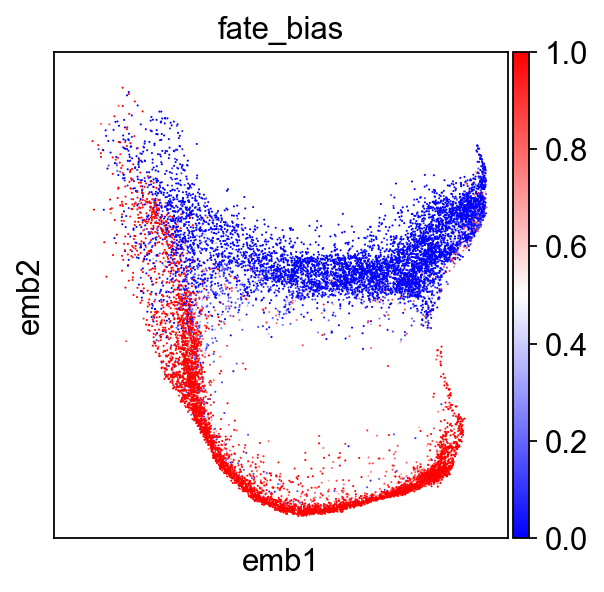
Let’s display our extracted fate biases
sc.pl.embedding(adata[(adata.obs.fate_bias-.5).abs().sort_values().index],
                color="fate_bias",basis="emb",sort_order=False,cmap='bwr')
Take home messages for efficient code writing and sharing
- Before attempting to parallelize every possible for loop, try to vectorize your code as much as possible. Numpy provides a wide range of fast functions for this purpose.
- Be mindful of data read/write and indexing, especially on slower HDD systems. Sometimes, pre-allocating data arrays and/or sorting indexes can be beneficial strategies.
- For actual computations occurring on large datasets, use Numba or Cython implementations whenever possible. Writing in Numba is particularly straightforward as its syntax is identical to Python’s.
- Don’t hesitate to explore the web or ask some LLMs. There’s a good chance someone has already implemented a particular subfunction you need!
- Identify the slow parts of your code by profiling the runtime line by line. A simple and effective tool for this task is line_profiler.
However, there’s an important caveat:
- Don’t waste your time optimizing a code/function that isn’t expected to be used frequently by you or other people. It’s crucial to assess where our time is best invested!